엑셀 평균 구하기: AVERAGE 함수 완전 정복과 평균이 틀리는 흔한 이유

엑셀 평균 구하기, 분명히 맞게 계산했는데 AVERAGE 결과가 다르다는 경험 한 번쯤은 있으실 겁니다.
함수가 잘못된 게 아닙니다. 대부분은 빈 셀, 0값, 텍스트, 가중치를 잘못 이해한 것이 원인입니다.
이 글에서는 엑셀 AVERAGE 함수의 기초부터 조건부 평균 AVERAGEIF·AVERAGEIFS, 그리고 흔히 틀리는 평균의 평균까지 차근차근 정리합니다.

AVERAGE 함수 기본 사용법과 범위 지정

기본 구문과 범위 입력 방식

엑셀 AVERAGE 함수의 기본 구문은 =AVERAGE(number1, [number2], ...)입니다. 첫 번째 인수는 필수이며 추가 인수는 최대 255개까지 넣을 수 있습니다.
가장 일반적인 사용법은 =AVERAGE(B2:B11)처럼 연속된 셀 범위를 지정하는 방식입니다. 범위 안의 숫자만 자동으로 평균에 반영되며, 셀 개수를 직접 세지 않아도 됩니다. 핵심은 AVERAGE가 숫자만 카운트한다는 점입니다. 범위에 텍스트가 섞여 있어도 숫자만 평균내므로, 수동 계산과 결과가 달라질 수 있습니다.

불연속 범위·여러 인수 지정하기

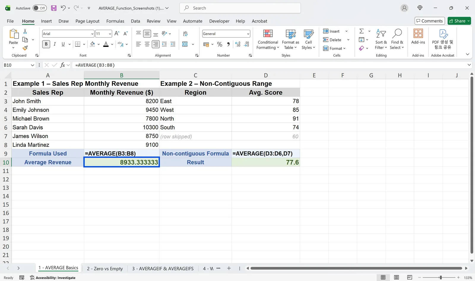
=AVERAGE(A1:A5, C1:C5, E1)처럼 떨어진 범위도 함께 계산할 수 있습니다. 단, AVERAGEIF와 AVERAGEIFS는 불연속 범위를 직접 다루지 못합니다. 필터링이 필요한 상황에서는 범위를 연속으로 구성하는 것이 안전합니다.

엑셀 평균 오류 원인 1순위: 0값과 빈 셀의 차이

빈 셀은 무시, 0은 포함됩니다

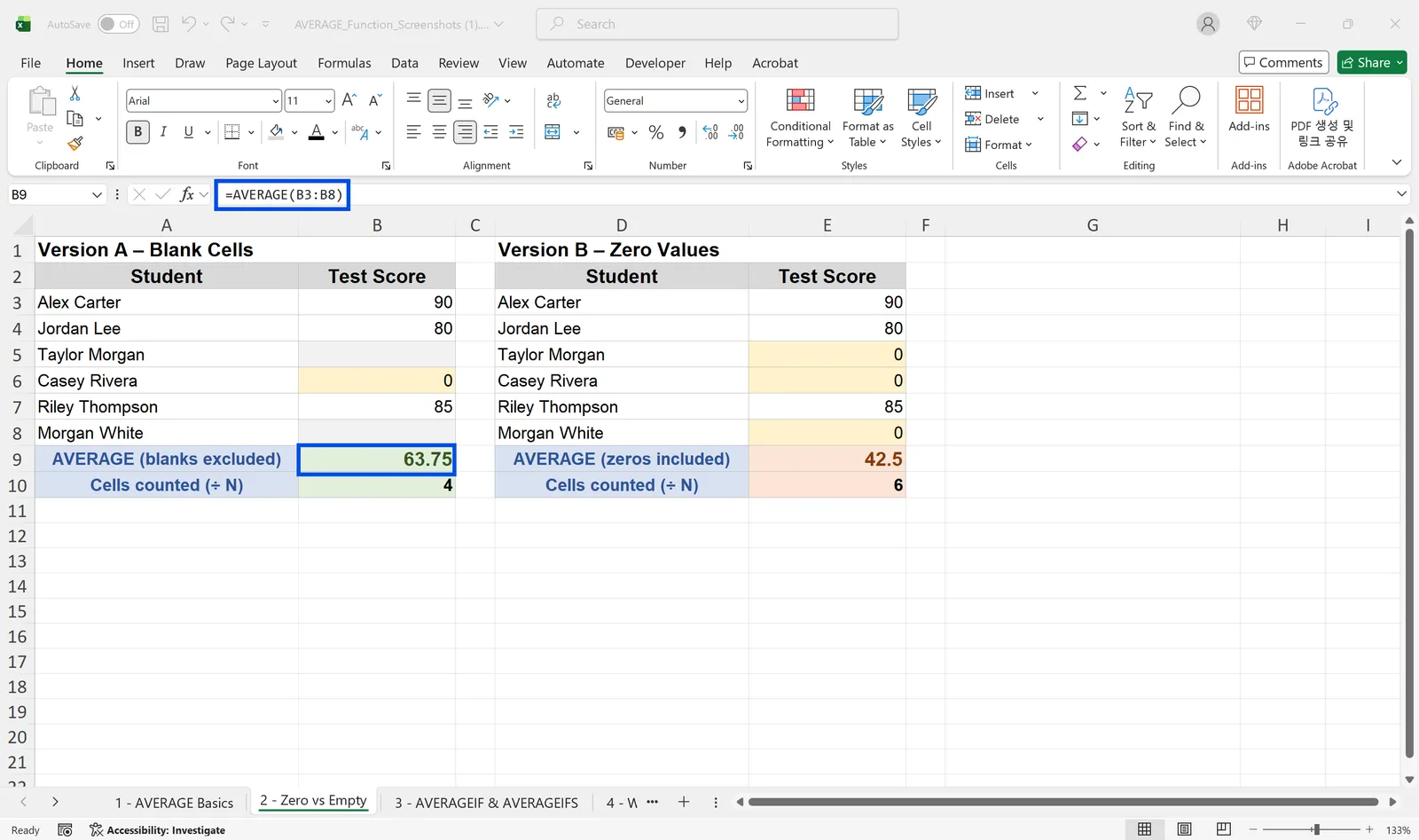
엑셀 평균 오류 중 가장 흔한 원인입니다. 빈 셀은 제외되고 0은 포함된다는 점을 놓치면 계산이 틀립니다. Microsoft 공식 문서에도 값이 0인 셀은 평균에 포함되지만, 빈 셀이나 텍스트는 무시된다고 명시되어 있습니다.
예를 들어 90, 80, 빈칸, 0이 있다면 AVERAGE는 빈칸을 제외하고 90, 80, 0만 계산합니다. 평균은 170÷3=56.7이 됩니다. 빈칸을 0처럼 생각하고 170÷4로 계산하면 42.5가 나와 값이 완전히 달라집니다.

엑셀 빈 셀 평균 제외 처리법

'미입력'과 '실제 0'은 의미가 다르므로 데이터 입력 단계에서 구분해 두는 것이 중요합니다. 엑셀 빈 셀 평균 제외가 필요할 때는 AVERAGEIF로 조건을 거는 방식이 가장 깔끔합니다. 0보다 큰 셀만 평균내려면 =AVERAGEIF(B2:B11,">0")처럼 조건을 걸면 됩니다. 빈 셀과 0을 동시에 제외할 수 있어 실무에서 자주 쓰이는 패턴입니다.

엑셀 조건부 평균: AVERAGEIF와 AVERAGEIFS 활용

엑셀 AVERAGEIF 단일 조건 사용법

AVERAGEIF는 하나의 조건에 맞는 셀만 평균내는 함수입니다. 기본 구문은 =AVERAGEIF(range, criteria, [average_range])입니다. average_range를 생략하면 range가 그대로 평균 대상이 되므로, 조건 범위와 평균 범위가 다를 때는 세 번째 인수를 반드시 명시해야 합니다.
예를 들어 =AVERAGEIF(A2:A10,"영업팀",B2:B10)은 A열이 '영업팀'인 행의 B열 평균을 구합니다. 조건에 맞는 값이 하나도 없으면 #DIV/0! 오류가 발생하므로, 데이터에 해당 조건이 실제로 있는지 먼저 확인하세요.

👉 엑셀 IF 함수 조건식 쉽게 이해하기 | 중첩 IF·오류처리(IFERROR) 완벽 정리

엑셀 AVERAGEIFS 다중 조건 사용법

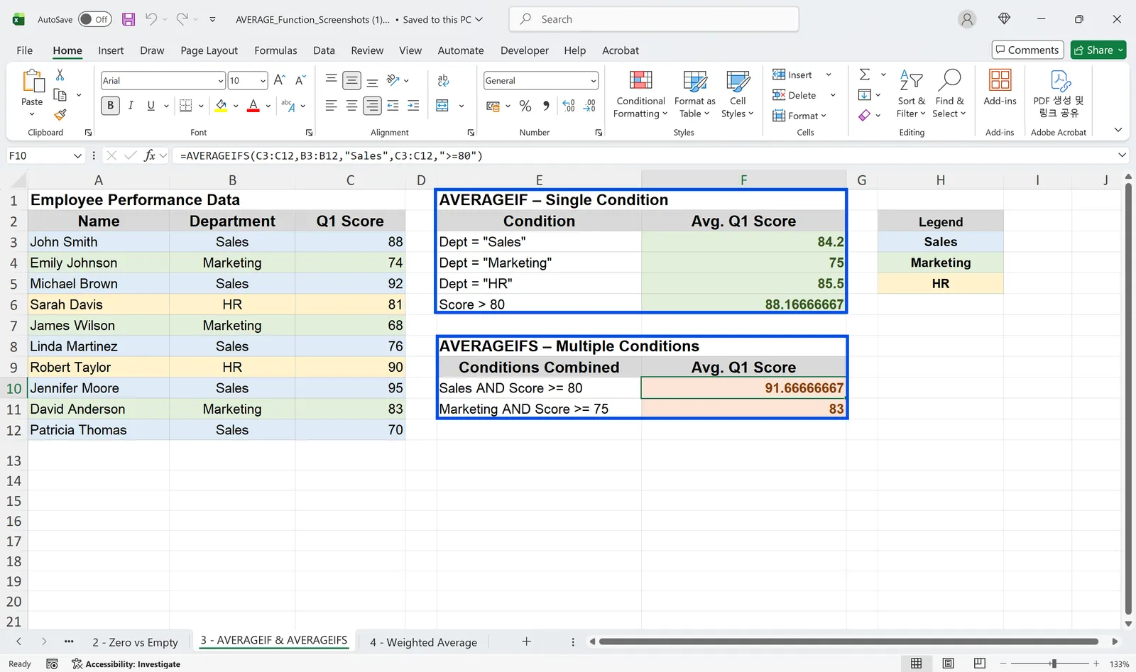
AVERAGEIFS는 여러 조건을 동시에 걸 수 있는 함수입니다. 구문은 =AVERAGEIFS(average_range, criteria_range1, criteria1, ...)이며, 기준 범위와 기준은 최대 127개까지 지정 가능합니다.
예를 들어 =AVERAGEIFS(C2:C100, A2:A100, "Sales", B2:B100, ">=80")처럼 부서와 점수를 함께 제한할 수 있습니다. '평균 낼 범위'와 '조건을 검사하는 범위'를 혼동하지 않는 것이 중요합니다. 또한 조건 범위의 빈 셀은 0으로 취급되므로, 조건은 맞는데 결과가 이상하다면 이 부분을 먼저 점검하세요.

평균의 평균이 틀리는 이유와 올바른 계산법

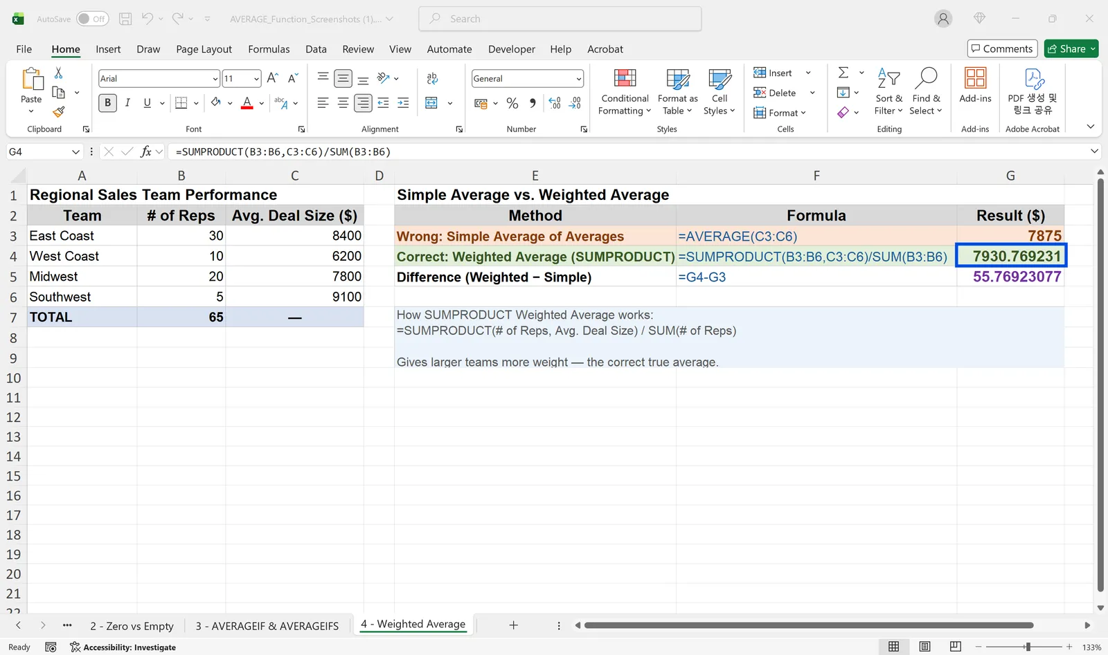
A팀 평균 80점, B팀 평균 60점을 단순히 더해 70점으로 묶으면 어떻게 될까요? 두 팀의 인원이 다르다면 실제 전체 평균과 어긋납니다. 이것이 평균의 평균이 틀리는 대표 원인입니다.
이럴 때는 가중평균이 필요합니다. 엑셀에서는 SUMPRODUCT와 SUM 조합이 가장 대표적인 방법입니다. 기본 수식은 =SUMPRODUCT(값범위, 가중치범위)/SUM(가중치범위)입니다. 값에 가중치를 곱해 합산한 뒤, 가중치 합으로 나누는 구조입니다.
예를 들어 A팀 30명(평균 80점), B팀 10명(평균 60점)이라면 단순 평균은 70점이지만, 가중평균은 (80×30 + 60×10)÷40 = 75점이 됩니다. 집단 크기가 다를 때는 반드시 가중평균을 사용해야 데이터를 왜곡 없이 분석할 수 있습니다.

👉 엑셀 데이터 필터 제대로 사용하는 방법 | 자동 필터·고급 필터 완벽 정리

엑셀 평균 구하기 AVERAGE 함수 자주 묻는 질문 (FAQ)

Q1. AVERAGE와 수동 합산 결과가 다를 때는 어떻게 확인하나요?

빈 셀, 텍스트, 0값을 먼저 확인하세요. 상태 표시줄의 '평균'과 '개수'를 함께 확인하면 어디서 차이가 생기는지 빠르게 파악할 수 있습니다.

Q2. 텍스트가 섞인 범위의 평균은 어떻게 처리하나요?

AVERAGE는 텍스트를 무시하고 숫자만 평균냅니다. '100' 같은 텍스트 형식 숫자가 섞여 있다면, VALUE 함수나 텍스트 나누기로 실제 숫자로 변환한 뒤 평균을 구해야 합니다.

Q3. #DIV/0! 오류는 어떻게 해결하나요?

조건에 맞는 데이터가 실제로 있는지 먼저 확인하세요. 화면 표시만 처리하고 싶다면 =IFERROR(AVERAGEIF(...), "해당 없음")처럼 IFERROR로 감싸면 됩니다.

inline AI로 엑셀 평균 작업 더 스마트하게

AVERAGE 함수를 익혔다면, 이제 반복 작업을 자동화할 차례입니다. 매번 AVERAGEIF 구문을 작성하고 조건 범위를 확인하는 시간을 줄이고 싶지 않으신가요?
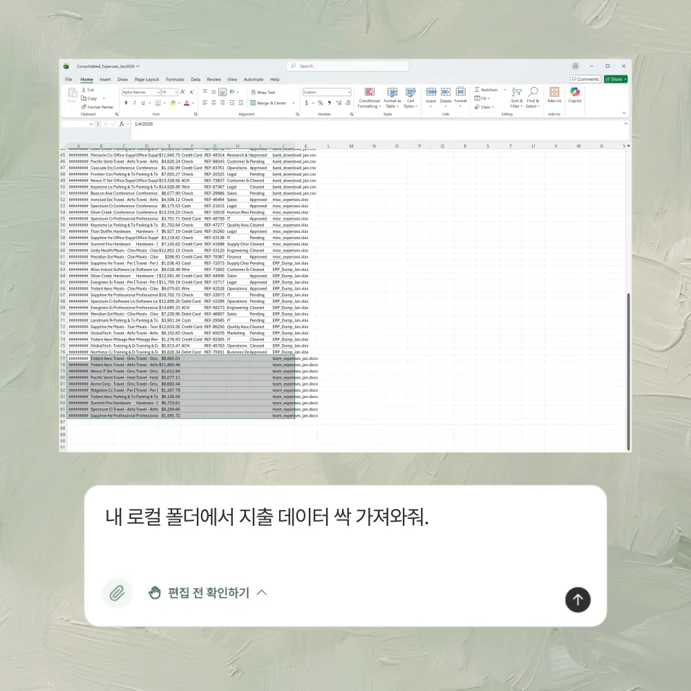
inline AI는 엑셀과 한글 문서 위에서 작업하는 최초의 로컬 에이전트입니다. ‘엑셀 표준편차 구해줘’처럼 자연어로 요청하면 Excel 파일을 직접 읽고 실시간으로 편집합니다.
데이터를 클라우드에 올리지 않고 PC에서 로컬로 작동해 민감한 데이터도 안전하게 처리합니다. 지금 바로 다운로드하고 엑셀 작업의 미래를 직접 경험해보세요.

👉🏻 inline AI 지금 바로 다운로드하기