Conditional Formatting in Excel: Highlight Cells, Whole Rows, and Banded Rows

Once a spreadsheet grows past a few hundred rows, finding the number that actually matters becomes a scrolling exercise. Conditional formatting in Excel solves that by changing a cell's color, font, or icon automatically based on its value or a formula. You set the rule once, and the formatting updates itself the moment your data changes.

This guide covers the practical ground: where to find the feature, how to highlight cells by value, text, or date, how to color an entire row with a formula, how to band alternating rows with MOD, and how to fix the rules that quietly refuse to fire.

Where Conditional Formatting Lives

Select the range you want to format, then go to the Home tab and click Conditional Formatting in the Styles group.

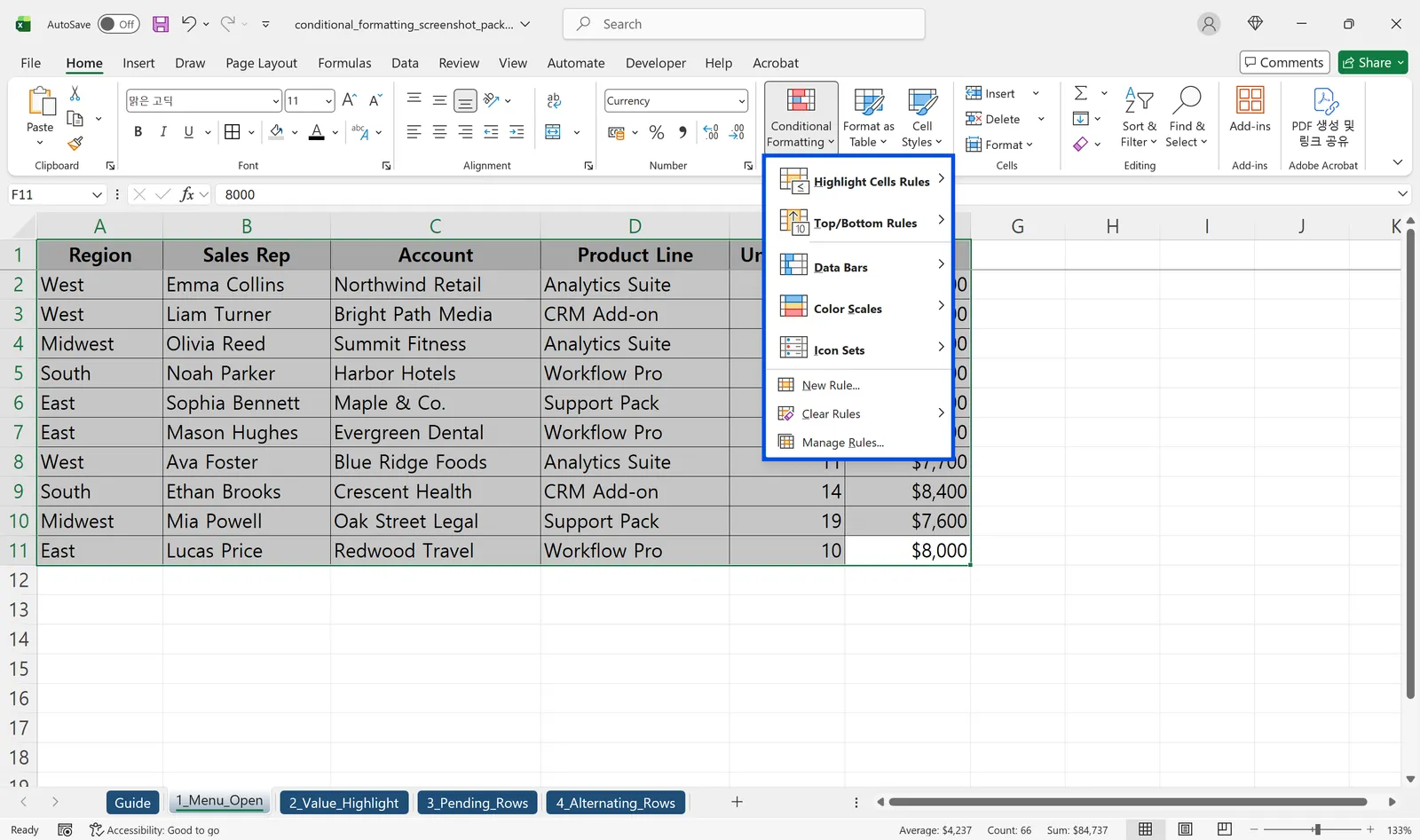
The dropdown is split into a handful of rule types:

• Highlight Cells Rules for greater than, less than, text that contains, dates, and so on
• Top/Bottom Rules for the top 10, bottom 10%, above average, and similar
• Data Bars, Color Scales, and Icon Sets for in-cell visualizations
• New Rule for custom formula-based logic, plus Clear Rules and Manage Rules

If you are new to this, start with Highlight Cells Rules and save the formula-based New Rule option for once the basics feel natural.

Highlight Cells by Value, Text, or Date

The fastest win is Highlight Cells Rules. Pick the type of comparison, type in your threshold, and choose a format.

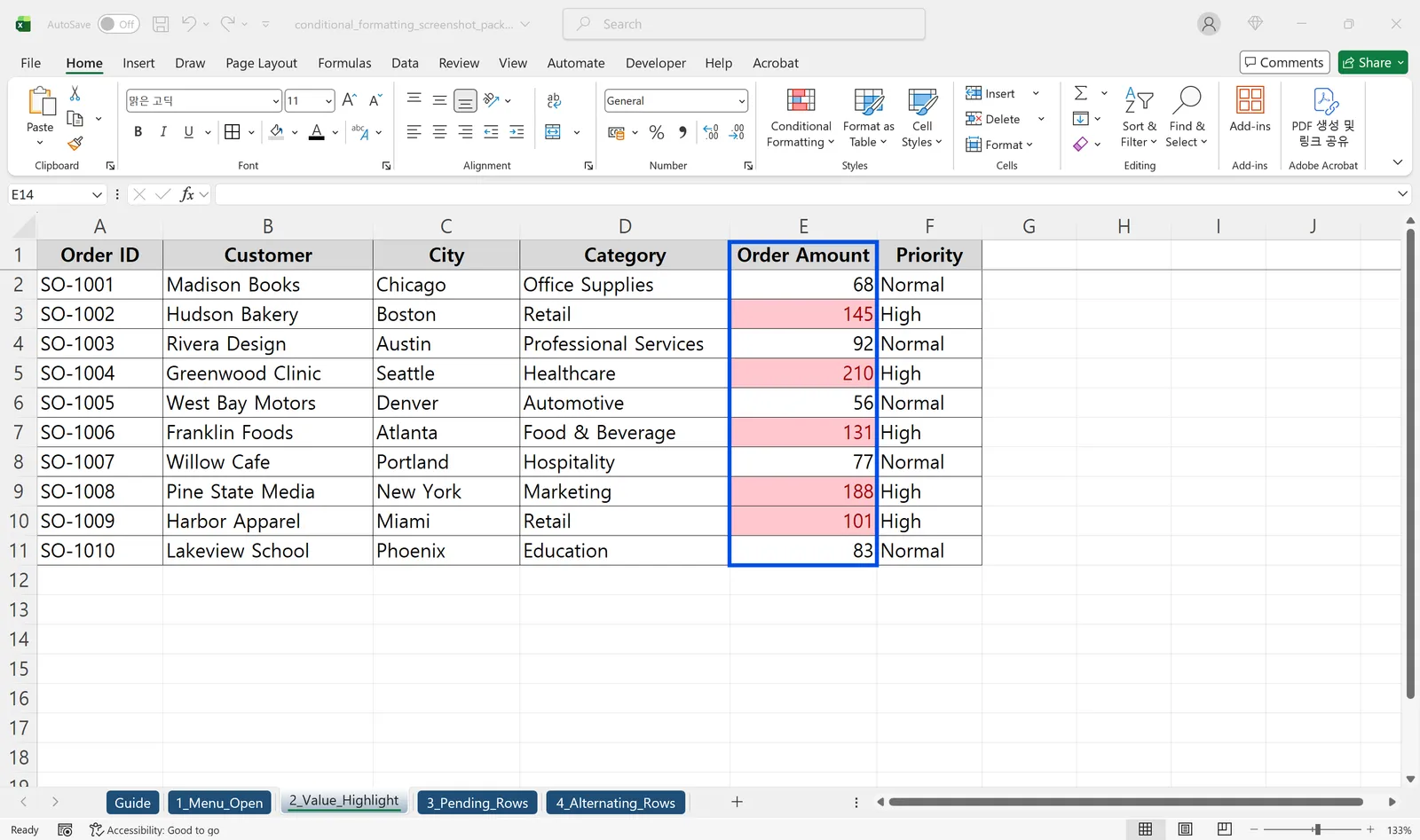
In the example above, the rule is Highlight Cells Rules > Greater Than with a threshold of 100. Every order amount over 100, such as 145, 210, and 188, turns red automatically, while values like 68 and 92 stay plain. Swap the hard-coded 100 for a cell reference like $C$1 and the highlight threshold updates the instant that reference cell changes.

The same menu handles the other common cases:

• Text that Contains flags any cell holding a keyword like Urgent, Error, or VIP, which is perfect for a status column.
• A Date Occurring offers ready-made options like Yesterday, Today, In the last 7 days, and This Week, all calculated against the current date.

For logic more complex than a single comparison, you move up to formula rules, which is exactly where the real power starts.

Highlight an Entire Row with a Formula

Coloring one cell is useful, but highlighting the whole row when a condition is met is what makes a table readable at a glance. This needs a formula rule.

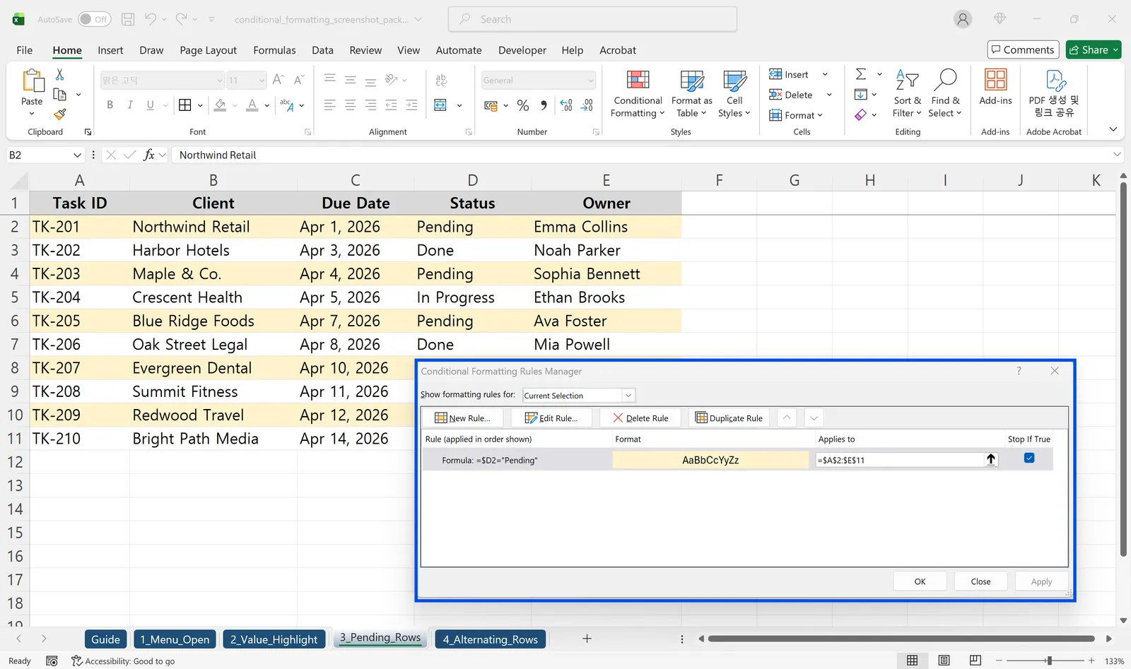
Say you have a task table with Status in column D. To shade every row whose status is Pending:

1. Select the full data range first, for example A2:E11 (headers excluded).
2. Go to Home > Conditional Formatting > New Rule > Use a formula to determine which cells to format.
3. Enter =$D2="Pending".
4. Pick a fill color and confirm.

Every row where column D reads Pending gets colored, and the moment a status changes to Done, its highlight clears itself.

The single most important detail here is the dollar sign. Writing =$D2 locks the column to D while leaving the row relative, so each row checks its own status. If you write =$D$2 instead, every row looks at cell D2 only, and the whole thing breaks. For combined conditions, the same kind of logic you would build with the IF function works inside the rule, for example =AND($D2="Delayed",$C2<TODAY()) to flag only overdue tasks.

Band Alternating Rows with MOD

Striped rows make wide tables far easier to read, and doing it by hand means redoing the work every time you add a row. A formula rule with MOD and ROW keeps the stripes automatic.

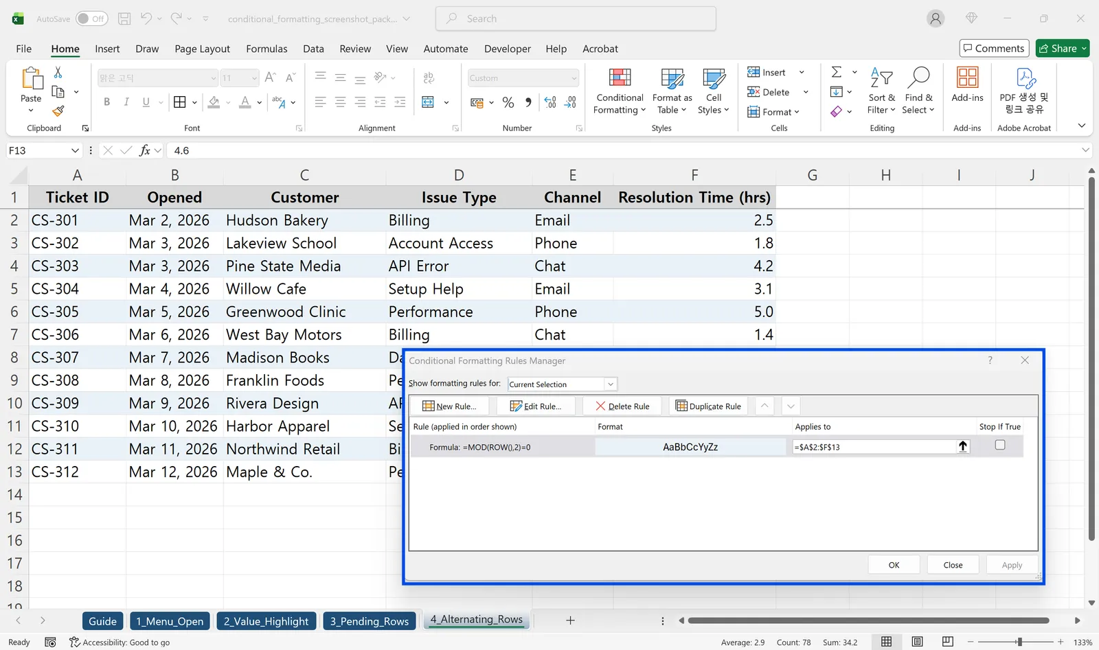
ROW() returns the current row number, and MOD(number, 2) returns the remainder after dividing by 2. Even rows have a remainder of 0, so =MOD(ROW(),2)=0 is TRUE on every even row and shades it.

1. Select your table range.
2. Go to Conditional Formatting > New Rule > Use a formula to determine which cells to format.
3. Enter the formula and choose a fill color.

Want to band every third row instead? Use =MOD(ROW()-2,3)=0. To alternate two colors, create two rules that test different remainders (0 and 1). Either way, the pattern recalculates itself whenever rows are added or deleted, so the banding never falls out of sync. This is the kind of clean, scannable layout that pairs well with Excel's filters when you are working through a large dataset.

When Conditional Formatting Does Not Work

If a rule looks right but the colors are missing or landing on the wrong cells, check these three things in order.

• Rule priority. When rules overlap on the same range, the one at the top wins. Open Conditional Formatting > Manage Rules, drag the more important rule higher, and use Stop If True to block later rules from interfering.
• Reference style. For whole-row rules, you want =$D2="value": column locked, row relative. A fully absolute =$D$2 makes every row read the same single cell, which is the most common reason row highlighting misbehaves.
• Applies to range. In Manage Rules, confirm the Applies to range actually covers your data. Start it at the first data row (not the header) and leave a little room for the table to grow.

Frequently Asked Questions

How many conditional formatting rules can I create?

It varies by version, but dozens to hundreds per sheet will work. Too many rules can slow recalculation, so consolidate identical patterns into a single rule with a wider range whenever you can.

Can I copy conditional formatting to other cells?

Yes. Select a formatted cell, click Format Painter (the paintbrush icon) on the Home tab, and drag across the target range to carry the rules along. You can also edit the Applies to range directly in Manage Rules.

Do the colors stay when I print?

Yes, fill and font colors print just like normal formatting. In black-and-white or grayscale printing the colors show up only as differences in shade, so check Print Preview first. If you are protecting a finished report, it also pairs well with locking specific cells.

Conditional Formatting Gets Easier with inline AI

Once you are comfortable with conditional formatting, the next step is to stop building the same rules by hand on every new file. Selecting ranges, getting the $ references right, and re-checking rule priority is exactly the repetitive setup that eats your time.

inline AI is the first local AI agent that works directly on top of your Excel and document files. Ask in plain English, like "highlight every row where status is Pending," and it reads the file, builds the rule, and applies it in real time, dollar signs and all.

Because it runs locally on your PC with nothing uploaded to the cloud, even sensitive data stays on your machine, and it ranks #1 on SpreadsheetBench with 92% accuracy.

Let inline AI handle the repetitive rule-building so you can focus on what your data is actually telling you.