

Blog
Conditional Formatting in Excel: Highlight Rows by Formula

Conditional formatting in Excel changes a cell's fill, font, data bar or icon automatically when its value meets a rule you set. On a 600-row stock sheet, scanning for the 20 items below safety stock takes ten minutes by eye; with one rule, they are red the moment the file opens, and they turn back to white when stock is replenished. No one has to repaint the sheet every Monday.
The menus are easy. The rules are where people get stuck: a whole-row highlight that colors the wrong rows because of one dollar sign, two rules fighting over the same cell, a range that stops ten rows short of new data. This guide covers the built-in rules, formula rules, rule order, and the fixes for each of those problems, then walks through a complete stock sheet setup.
Where conditional formatting lives in Excel
Select the range first, then go to Home > Styles > Conditional Formatting. Microsoft's support article on conditional formatting groups the options into the same families you see in the menu.
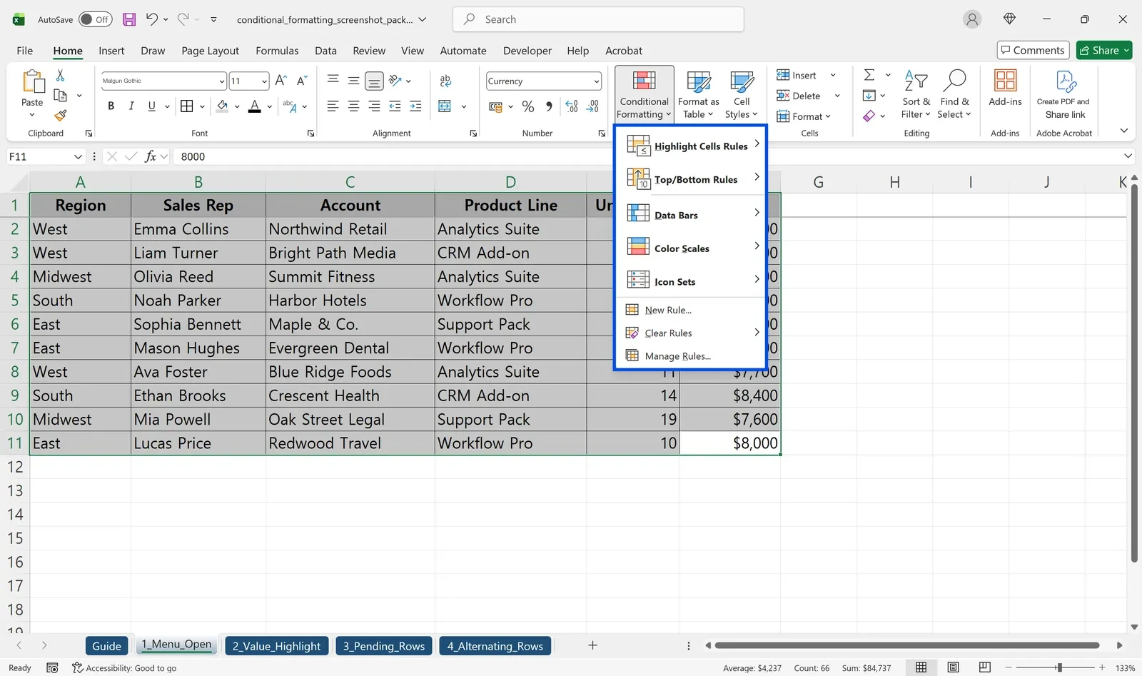
| Menu | Conditions you can pick | Typical use in a distribution or manufacturing office |
|---|---|---|
| Highlight Cells Rules | Greater Than, Less Than, Between, Equal To, Text that Contains, A Date Occurring, Duplicate Values | Open invoices over $10,000, orders marked "Hold", duplicate PO numbers |
| Top/Bottom Rules | Top 10 Items, Top 10%, Bottom 10 Items, Bottom 10%, Above Average, Below Average | Top customers by revenue, lines with above-average scrap |
| Data Bars | A bar inside the cell sized to the value | Comparing on-hand quantity across SKUs |
| Color Scales | A two- or three-color gradient from low to high | A heat map of monthly shipments |
| Icon Sets | Arrows, traffic lights, flags | Month-over-month change |
Anything the menus don't offer goes through New Rule > Use a formula to determine which cells to format. In practice, "color the whole row" and "color this cell based on another column" are both formula rules.
Highlight cells by value, text or date
Start with Highlight Cells Rules. Select the order amount column, choose Greater Than, enter 100, and every amount over 100 turns light red.
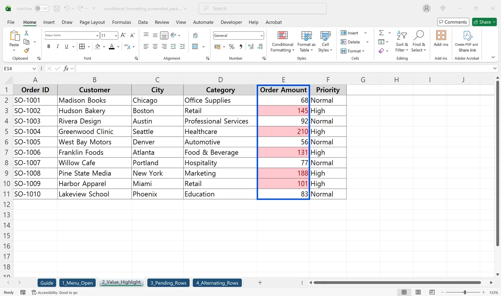
Instead of a typed number, put a cell reference such as $C$1 in the value box. Now the threshold lives on the sheet, and changing it in C1 updates the highlighting without opening the rule again. Text that Contains flags words like Urgent or Return, and A Date Occurring handles Yesterday, Today, Last 7 days, This Month and similar windows.
Highlight an entire row with a formula
To color a whole row based on one column:
- Select the data without the header row, for example
A2:H600, starting from A2. - Go to Conditional Formatting > New Rule > Use a formula to determine which cells to format.
- In Format values where this formula is true, enter
=$D2="Pending". - Click Format, choose a fill, and click OK.
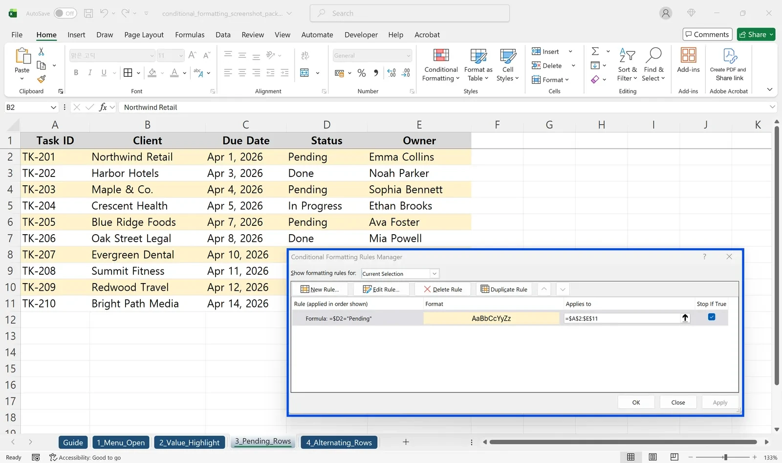
The dollar sign does all the work. Excel writes the formula relative to the active cell of your selection (A2 here) and shifts it for every other cell in the range. $D2 locks the column to D but lets the row move, so every cell in row 2 checks D2, every cell in row 3 checks D3, and so on. Write $D$2 and all 600 rows check the same cell, so either everything is colored or nothing is. Write D2 with no dollar sign and column B checks E, column C checks F, and you get a strange stripe pattern.
The formula must return TRUE or FALSE. Combine conditions with AND or OR, for example =AND($D2="Pending",$F2<TODAY()) for pending shipments past their promised date. You can also point at another sheet, as in =$B2<>PriceList!$B2, which is how many people compare two versions of a price list.
Band alternating rows
=MOD(ROW(),2)=0 is TRUE on even rows, so they get shaded. Microsoft's guide to applying shading to alternate rows uses the same formula.
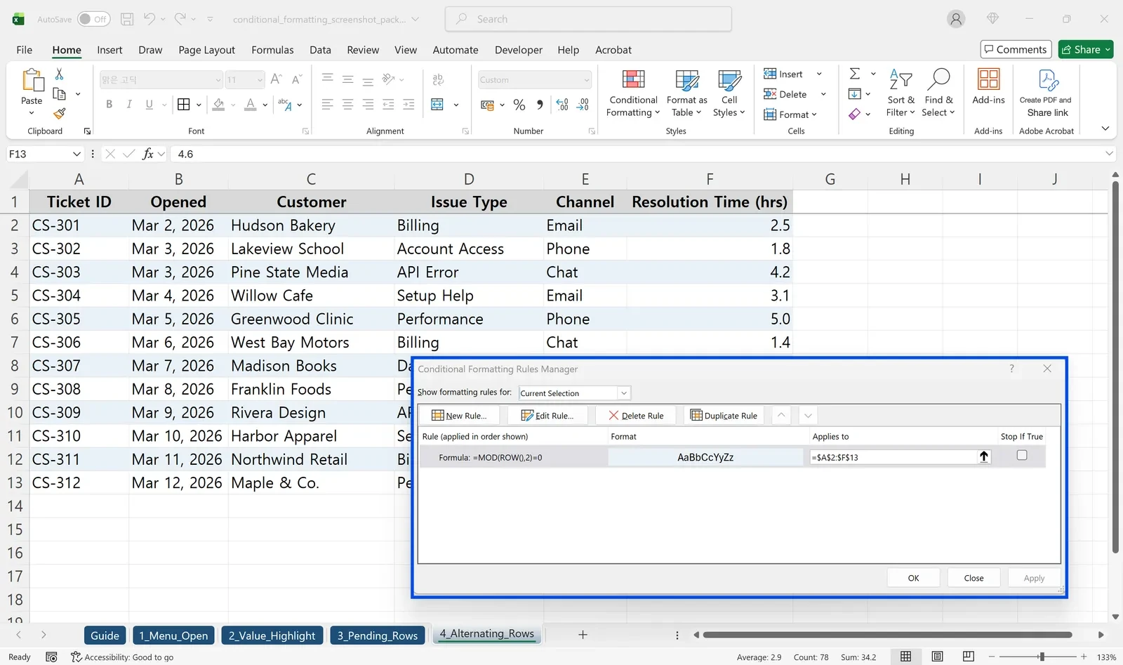
Hand-painted bands break as soon as someone inserts a row. This rule recalculates from the row number, so the bands stay correct. For every third row, use =MOD(ROW()-2,3)=0. If you can convert the range to a table with Home > Format as Table, the Banded Rows option does the same thing without a rule.
Data bars, color scales and icon sets
These are better than on/off colors when the point is comparing sizes. Data bars turn a quantity column into an in-cell bar chart; in Edit Rule, tick Show Bar Only to hide the numbers. Color scales shade from low to high, which works well for a grid of defects by line and month.
Icon sets default to percent thresholds (67% and 33%). For a metric with a fixed target, such as fill rate against 100%, open Edit Rule, change the type to Number, and type the cutoffs yourself: green at 1 or above, yellow at 0.8 or above, red below that. The icons then mean the same thing every month, no matter how the data shifts.
Worked example: a weekly stock check at Northgate Supply
The warehouse lead at Northgate Supply reviews the stock sheet every Monday. Columns are SKU (A), Item (B), Lot (C), Available (D), Safety Stock (E), Expiry Date (F), Last Shipped (G) and Location (H), with data in rows 2 to 600. Three questions matter: what needs reordering, which lots are close to expiry, and what hasn't moved in three months.
1. Create four rules
With A2:H600 selected, add these formula rules:
- Expired lot:
=$F2<TODAY(), dark red fill with white font - Below safety stock:
=$D2<$E2, light red fill - Expiring within 30 days:
=AND($F2>=TODAY(),$F2<=TODAY()+30), orange fill, applied toF2:F600only - No shipments for 90 days:
=TODAY()-$G2>90, gray font
Keeping the expiry rule on column F means a row can carry two signals at once: the row color says "reorder" and the date cell says "expiring soon".
2. Check the rule order
Open Conditional Formatting > Manage Rules and set Show formatting rules for to This Worksheet. This is where you find last quarter's "red if zero" rule that only covers A2:H350. Delete duplicates, merge rules that were split across ranges, and move the expired-lot rule to the top.
3. Spot-check the result
Pick two colored rows and one plain row and compare the numbers by eye. Blank Available cells count as zero, so they show as below safety stock; if that's wrong for your sheet, use =AND($D2<>"",$D2<$E2). Dates imported as text won't compare to TODAY() and stay uncolored, so fix the date column first if it's left-aligned.
4. Filter by color to build the reorder list
Colors from conditional formatting work with Filter by Color. Turn on filters, open the Available column, filter by the light red fill, and only the items to reorder remain. Sort by supplier and you have the day's purchase list.
👉 How to Filter Data in Excel: AutoFilter and Advanced Filter
When a conditional formatting rule doesn't work
The rule precedence section of Microsoft's conditional formatting article explains the order: rules higher in the list are evaluated first, and a new rule is added at the top by default, so the rule you made last wins unless you move it. If two rules don't conflict (one sets bold, the other sets a fill), both apply. If they do conflict (both set a fill), the higher rule wins. Most broken rules come down to one of these:
- Every row or no row is colored. The formula locks the row (
$D$2). Remove the dollar sign before the row number. - Colors are shifted by one row. The range was selected bottom-up, so the active cell was A600. Reselect from A2 and write the formula for row 2.
- Only the top rule's color shows. Two fill rules overlap. Reorder them in Manage Rules or tick Stop If True.
- New rows have no color. Applies to stops at the old last row. Extend it, or convert the range to a table with Ctrl+T so the rule grows with the data.
- Number or date comparisons fail. The values are stored as text. Convert them to numbers or dates.
Copy and paste quietly multiplies rules. Pasting formatted cells elsewhere, or cutting and moving rows, splits one rule into several with different ranges, and a file with dozens of fragments scrolls slowly. Merge them in Manage Rules once a quarter, and use Paste Special > Values when you only need the numbers.
To remove rules, use Clear Rules > Clear Rules from Selected Cells or Clear Rules from Entire Sheet. The second also removes everyone else's rules, so look at the Rules Manager first.
Version differences
Microsoft 365, Excel 2021, 2019 and 2016 for Windows share the same menus. Selecting a range also shows the Quick Analysis button (Ctrl+Q), whose Formatting tab applies data bars, color scales and Greater Than in one click. Excel for the web has Home > Conditional Formatting with the same rule types, and Excel for Mac puts the formula option under New Rule > Style: Classic. The old Excel 97-2003 format (.xls) keeps only three conditions per cell, so save rule-heavy sheets as .xlsx.
FAQ
Q. Can I copy conditional formatting to another range or file?
Yes. Select a formatted cell, click Format Painter on the Home tab, and drag across the target range; the rule comes with it. The same works between workbooks, but if the formula refers to another sheet, the target workbook needs a sheet with the same name.
Q. Can one cell's color depend on a different column?
Yes, with a formula rule. Select column C and use =$E2="Return", and each C cell is colored when its row's E value is "Return".
Q. Do conditional formatting colors print?
They print like any other fill. On a black-and-white printer they become gray shades, so add bold text or icons to anything that must survive a photocopy.
Q. Do TODAY-based rules update by themselves?
Yes. TODAY() recalculates whenever the workbook opens or recalculates, so an expiry rule shows a fresh 30-day window every day.
How inline AI handles conditional formatting
With the stock sheet open, you tell inline AI something like "red for rows below safety stock, orange for lots expiring within 30 days," and it writes the formula rules and cleans up older rules that overlap. With ARP, items that drop below safety stock don't just turn red: inline AI sends the purchase order to the supplier.
Hand your documents and your company’s work to inline AI.
Keep a file open, say what you need, and AI edits it or drafts a new one. Add the company AI OS and AI runs the rest of the work, ERP included.
Book a demo