Learn
How to Fix Excel Formula Errors: #VALUE!, #REF!, #NAME?, #DIV/0!

Wrapping a #VALUE! cell in IFERROR is not fixing an Excel formula error. The message disappears from the screen, but the calculation underneath is still wrong, and now nobody can tell.
The good news is that Excel only has about eight error codes, and each one points at a fairly specific cause. Read the code correctly and you have already narrowed the problem down to one or two things.
This guide walks through how to fix Excel formula errors code by code, starting with the four you will actually meet at work: #VALUE!, #REF!, #NAME?, and #DIV/0!. It also covers the cases that are not error codes at all, such as a formula that displays as plain text, calculation stuck on manual, circular reference warnings, and the less common #SPILL! and #NUM!.
Excel Error Codes at a Glance
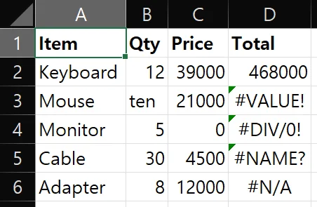
An error code is Excel telling you it started the formula and could not finish it. Which code you get depends on where the calculation stalled.
The eight codes and what triggers them
| Error code | Cause |
|---|---|
| #VALUE! | Text or a stray space sits where a number belongs |
| #REF! | A referenced cell, row, column, or sheet was deleted |
| #NAME? | Misspelled function, missing quotes, or an undefined name |
| #DIV/0! | Dividing by zero or by an empty cell |
| #N/A | VLOOKUP, MATCH, or XLOOKUP could not find the value |
| #NUM! | The math runs, but the result cannot be expressed as a number |
| #SPILL! | A dynamic array has no room to spill its results |
| #NULL! | A space between ranges produced no intersection |
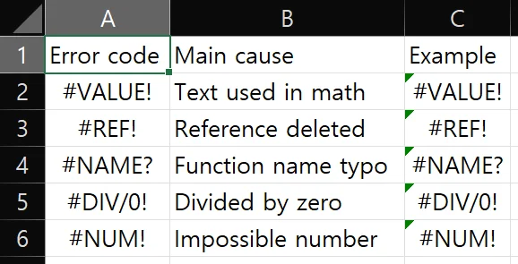
Seeing each code next to the result its example formula produces makes the pattern obvious. In everyday spreadsheets, four of them account for nearly all the damage: #VALUE!, #REF!, #NAME?, and #DIV/0!.
That green triangle is not an error
The small green triangle in the top-left corner of a cell is a different animal. It comes from Excel's background error checking, which is flagging something as suspicious. The formula itself ran fine.
The most common trigger by far is a number stored as text. You will also see it on a cell whose formula differs from its neighbors, or a cell that appears to have been left out of a nearby range.
If the triangles bother you, go to File > Options > Formulas and uncheck the relevant rule under Error checking rules. Just remember that switching off the warning and fixing the cause are two separate jobs.
Errors versus formulas that never calculated
Cells misbehave in three broadly different ways, and each needs a different approach.
- An error code appears. The formula ran and hit a wall. Identify the code, fix the cause.
- The formula shows as literal text. It never ran at all. This is a formatting or calculation-option problem.
- The result is always 0. It ran, but the values it referenced were probably not recognized as numbers.
Fixing #VALUE! Errors
#VALUE! is a data type mismatch. Excel expected a number, found text, and gave up.
Text and hidden spaces where numbers should be
The classic case is a unit typed into a quantity or amount cell. If someone entered 5 ea or 12,000 USD instead of 5 and 12000, any multiplication or addition against that cell breaks immediately.
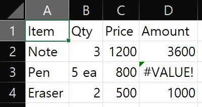
Often you cannot see the problem at all. A leading or trailing space, or a non-breaking space like CHAR(160) pasted in from a web page or an exported system report, looks identical to nothing on screen but stops arithmetic dead.
Three functions clean this up. TRIM strips leading and trailing spaces, CLEAN removes non-printing characters, and if something still survives both, target it directly with =SUBSTITUTE(A2,CHAR(160),"").
Converting numbers stored as text
If a cell was formatted as Text before the number was typed in, that number is stored as a string. Changing the format afterward does not convert the value on its own.
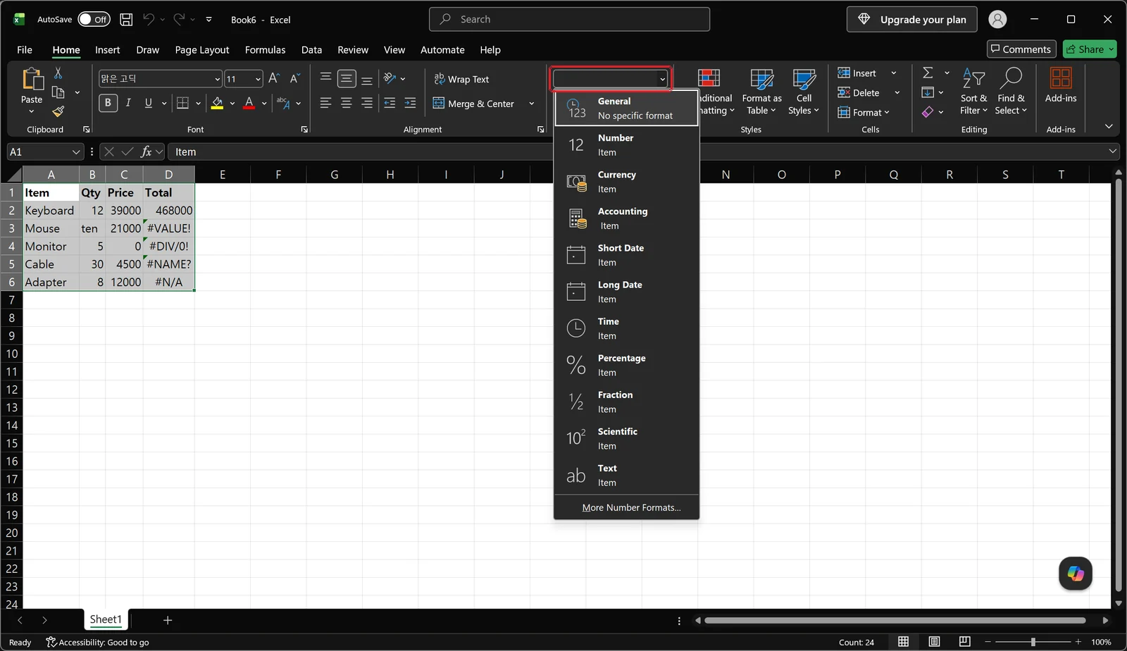
To convert text numbers back to real numbers:
- Select the range.
- On the Home tab, open the number format gallery and choose General.
- Press
F2on each cell to enter edit mode, then pressEnterto re-commit it.
Skip step 3 and you have changed the formatting while the value stays text. For a large range, select the whole column, go to Data > Text to Columns, and click Finish without changing a single setting. Excel re-enters every cell at once.
When dates are the ones stuck as text, DATEVALUE converts them into real date serial numbers.
👉 Excel Date Format Not Changing? Fix Serial Numbers, Text Dates, and DATEDIF
Working around it with SUM, VALUE, and TRIM
Sometimes you are not allowed to touch the source data. In that case, change the formula instead. Arithmetic operators like +, -, *, and / throw #VALUE! the moment they touch text, but SUM simply ignores text inside a range and adds the numbers.
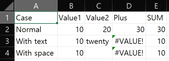
Rewriting =A2+B2 as =SUM(A2:B2) clears the error surprisingly often. Be careful, though: the ignored text is not counted. If that value was supposed to be part of the total, your result is now quietly wrong rather than loudly broken.
To actually convert the string and keep it in the math, wrap it: =VALUE(TRIM(A2))*B2 strips the spaces and casts the text to a number in one step.
Fixing #REF!, #NAME?, and #DIV/0!
These three have nothing in common except that they all look alarming. #REF! means the target is gone, #NAME? means Excel did not recognize a word in your formula, and #DIV/0! means the denominator is zero.
#REF! - recovering a deleted reference
#REF! appears when a cell, row, column, or sheet a formula pointed to gets deleted. Delete column C while =B2*C2 exists and the formula rewrites itself as =B2*#REF!.
If it just happened, Ctrl+Z is the cleanest fix. Undoing the deletion restores the reference and the formula returns to normal.
Once the file has been saved and closed, there is no automatic way back. You have to work out what the formula was pointing at and rewrite it.
To prevent it, convert your data range to a table with Ctrl+T and use structured references, or build formulas with INDEX so they do not depend on a hard-coded column position.
#NAME? - check the spelling, the quotes, and the names
#NAME? means Excel could not interpret some text in your formula as a function or a defined name. Run through this list and you will usually catch it on the first or second item.
- Misspelled function name such as
SUMM,VLOOKUPP, orAVERAG - Missing double quotes around text, as in
=IF(A2=Complete,1,0) - A deleted defined name that a formula still references after you removed it in Name Manager
- A function your version does not have, such as opening an
XLOOKUPworkbook in an older release - A missing colon, as in
=SUM(A2A10)instead of=SUM(A2:A10)
Type three letters of a function name and Excel's autocomplete list appears. Selecting from the list with Tab instead of typing the whole name out eliminates most of these errors before they happen.
#DIV/0! - zero and empty denominators
This one has exactly one cause: the divisor is zero, or the cell holding it is empty. Excel treats a blank cell as 0 in arithmetic, so both situations produce the same error.
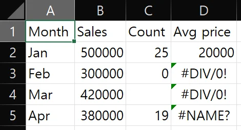
It shows up constantly when you build average or unit-price formulas ahead of the data. The fix is to test the denominator first:
=IF(C2=0,"-",B2/C2)
Choose the fallback based on who reads the sheet. A dash, an empty string, or a short label like No data all work, and a label makes it much easier for a reader to see why the cell is empty rather than assuming the number is zero.
Using IFERROR to Blank Out Error Values
Some errors survive even after you fix every cause, simply because of how the data behaves. IFERROR controls what appears on screen in those cases.
Syntax and how to retrofit it
The syntax has only two parts:
=IFERROR(original_formula, value_if_error)
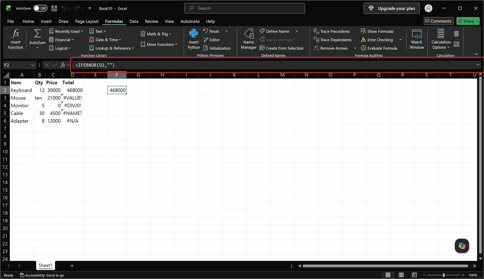
If the original formula works, its result passes through unchanged. If it errors, the second argument shows instead. For a blank cell, use two double quotes: =IFERROR(B2/C2,"").
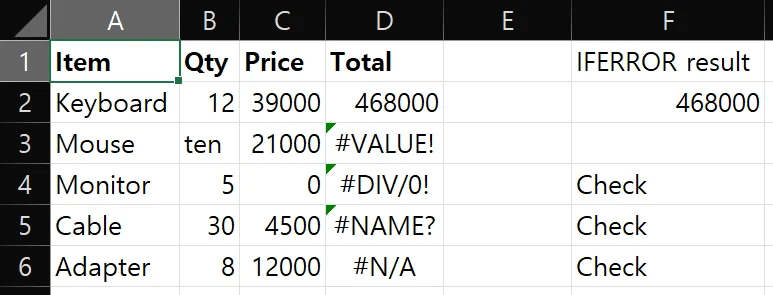
To add it to a formula you already wrote, type IFERROR( right after the equals sign and append ,"") at the very end.
IFERROR versus IFNA
IFERROR catches everything. Not just #N/A, but #REF!, #NAME?, and #VALUE! too, all replaced with whatever you specified.
That is precisely the danger. A broken reference or a mistyped function name gets painted over with a tidy blank, the sheet looks finished, and the report goes out with nobody aware the formula is dead.
If all you want to handle is a lookup that found nothing, IFNA is the safer choice. =IFNA(VLOOKUP(...),"Not registered") suppresses #N/A only and leaves every other error visible.
The working rule: apply IFERROR to formulas you have already verified, never to formulas you are still building.
Choosing between blank, 0, and a text label
The right replacement depends entirely on what happens to that cell next.
| Replacement | Good for | Watch out for |
|---|---|---|
"" (blank) | Printouts and summary tables you share | It is an empty string, not an empty cell, and downstream math may read it as 0 |
0 | Cases where including zero in a total is correct | "No value" and "zero" become indistinguishable |
"Check needed" | Rows that need someone to follow up | Text cannot be used in numeric calculations |
A cell holding "" looks empty but is not. ISBLANK returns FALSE for it and COUNTA counts it as populated, while COUNTBLANK does count it as blank - so the number you get depends on which function you ask. A chart may plot it as zero.
If you want the errors visible while you work but hidden on paper, go to Page Layout > Page Setup > Sheet and set Cell errors as to <blank>.
When Formulas Show as Text Instead of Results
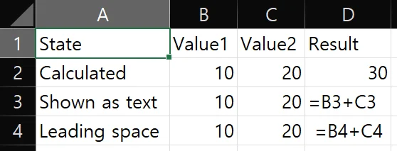
If a cell displays =B3+C3 literally rather than a number, this is not an error code at all. The formula never executed, and the cause is almost always one of four things.
The cell was formatted as Text
Enter a formula into a cell already formatted as Text and Excel stores it as a string. Left-aligned formula text is the giveaway.
Set the number format back to General on the Home tab, then press F2 on the cell and Enter. The re-entry is what makes Excel finally read it as a formula.
For a whole column, select it, run Data > Text to Columns, and click Finish without touching any options. It re-commits every cell in one pass.
Show Formulas mode is on
If every formula on the sheet turned into text at once, and the columns also got wider, you are in formula view.
Press `Ctrl+`` (the backtick key left of the 1) to toggle it off. The Show Formulas button in the Formula Auditing group on the Formulas tab does the same thing.
Calculation is set to Manual
If results refuse to update when you change the inputs and keep showing the old numbers, check the calculation mode. Large workbooks and files inherited from other people are often set to manual.
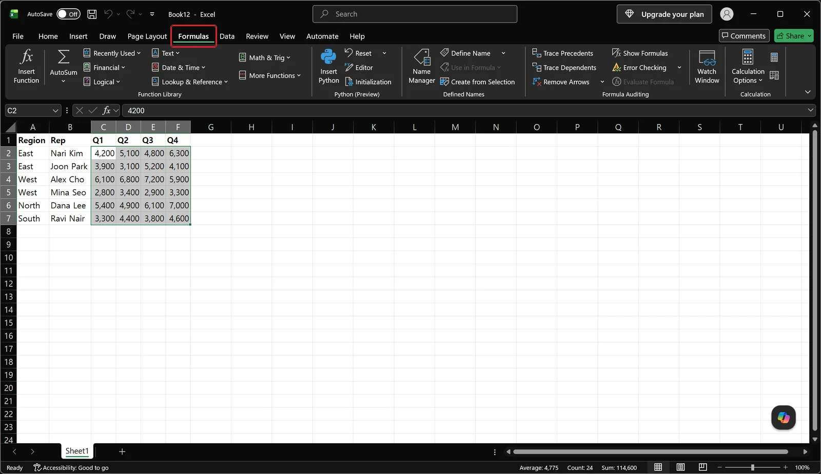
On the Formulas tab, open Calculation Options in the Calculation group and switch it to Automatic. For a one-off recalculation, press F9; to recalculate only the active sheet, press Shift+F9.
A leading space or apostrophe
A single space before the = makes Excel treat the entire entry as text. Click into the formula bar and move the cursor to the very start to check.
A leading apostrophe (') does the same thing and is harder to spot, because it never appears in the cell itself, only in the formula bar. In both cases, delete the character and press Enter.
👉 How to Copy Formulas in Excel | Fix Errors, Lock Cells with $, Use F4
Circular References, #SPILL!, and #NUM!
These come up less often than the big four, but they are the ones that leave people staring at the screen the first time.
Locating a circular reference
A circular reference happens when a formula refers to the cell it lives in. Putting =SUM(C1:C10) in cell C10 is the textbook example.
Excel throws a warning dialog, and even after you dismiss it, the status bar at the bottom left keeps showing Circular References along with the offending cell address.
If it spans several cells and you cannot find them all, go to Formulas > Error Checking > Circular References for the full list. Nine times out of ten the total cell got swallowed by its own sum range, and shrinking the range by one row fixes it.
#SPILL! - clearing the spill range
#SPILL! means a dynamic array formula wants to write results across multiple cells and something is already sitting there. You will see it with UNIQUE, FILTER, SORT, and SEQUENCE.
Select the error cell and Excel outlines the intended spill range with a dashed border. Delete or move whatever is inside that outline and the results fill in instantly.
Merged cells overlapping the range cause the same error, and the only fix is to unmerge them. Formulas that reference an entire column can also trigger it by trying to spill more than a million rows, so narrow the reference to the range you actually need.
#NUM!, #NULL!, and #N/A
#NUM! means the formula is structurally valid but the result cannot be represented as a number. Undefined math like =SQRT(-1), values beyond what Excel can hold, and iterative functions such as IRR or RATE that fail to converge all land here. Check the signs and units of your inputs first.
#NULL! appears when you put a space between two ranges that do not intersect. Almost always it is a missing comma, as in =SUM(A1:A5 C1:C5), so check your separators.
#N/A simply means the value was not found; the formula itself is fine. Work through the usual suspects in order: stray spaces in the lookup value, numbers stored as text, and a VLOOKUP fourth argument left as TRUE when you needed an exact match. To tidy up the display only, wrap it in IFNA.
Error Checking and Evaluate Formula
In a deeply nested formula, spotting the broken piece by eye is hopeless. The Formula Auditing group on the Formulas tab exists for exactly this.
- Evaluate Formula - steps through the formula, replacing each part with its actual value. The step where the error first appears is your culprit.
- Trace Precedents - draws arrows to the cells the current cell depends on.
- Trace Dependents - does the reverse, showing which cells rely on this one. Useful before you change a value.
- Error Checking - sweeps the sheet and jumps you from one problem cell to the next.
Frequently Asked Questions
Q. How do I remove all Excel error indicators at once?
It depends on what you actually want gone. To change the cell values themselves, wrap the formulas in IFERROR. To remove only the green triangles, go to File > Options > Formulas and uncheck the relevant rule under Error checking rules. To hide errors on printouts alone, set Cell errors as to <blank> under Page Layout > Page Setup > Sheet. Hiding without fixing means the document can be signed off while the math is still wrong, so verify the numbers before you suppress anything.
Q. What is the difference between #N/A and #VALUE!?
#N/A means a lookup function like VLOOKUP or MATCH searched and found nothing. The formula is working correctly and reporting an absence, so check the source list or clean up the display with IFNA. #VALUE! means the data types do not match and the calculation could not even begin. That one requires fixing the text or spaces in the referenced cells.
Q. Why does my formula keep returning 0?
The most common reason is that the referenced numbers are stored as text, so SUM skips all of them. Check whether the numbers are left-aligned, and run COUNT and COUNTA over the same range: different results mean text numbers are mixed in. Other possibilities are calculation set to manual, a number format with zero decimal places rounding small values out of sight, a condition that is always false, or a reference pointing at the wrong column.
Q. Is there ever a reason not to use IFERROR?
Yes, while you are still testing a formula. IFERROR masks signals like #REF! and #NAME? that mean the formula itself is broken, so a dead reference renders as a neat blank cell. If your only goal is to handle failed lookups, use IFNA, which catches #N/A and nothing else. Save IFERROR for formulas you have already confirmed are correct.
Checking Excel formula errors with inline AI
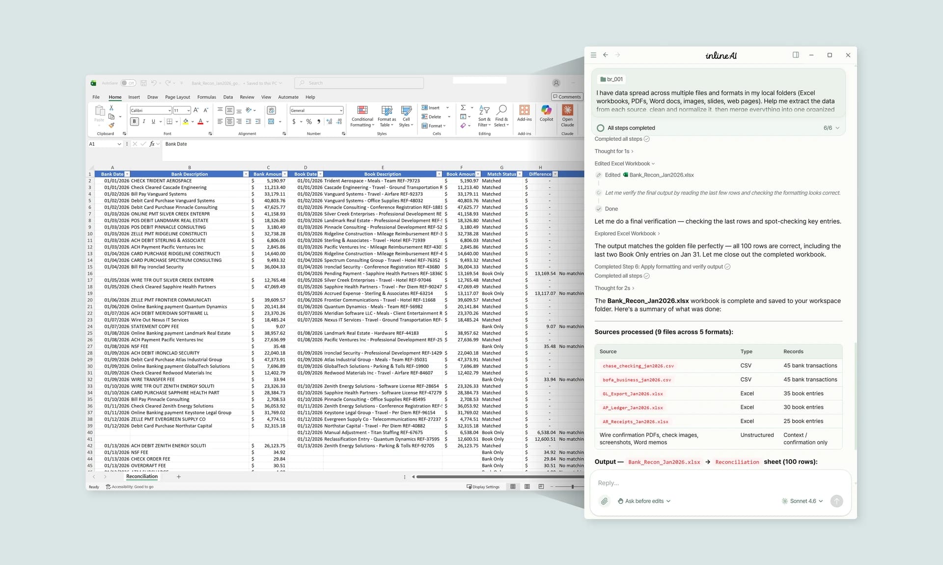
Even when you know what every error code means, tracking down which cell and which reference broke across a few hundred rows still takes time, and Evaluate Formula and reference tracing both work one cell at a time.
inline AI is a desktop AI tool that reads your Excel file directly. Ask it something like "find the cause of the #VALUE! errors in column D" and it locates the affected cells, explains why they failed, and corrects the formulas. It can also handle the repetitive parts, such as converting text-stored numbers across a range or applying IFERROR to a verified block of formulas.
It runs on your PC rather than uploading the file to a cloud service, so it works on internal data that is not allowed to leave the machine.
See what an agent could take over at your company in a 30-minute call.